Implementing non-integer Factorial and Gamma function for BigDecimal

Introduction

This article describes how the factorial and Gamma functions for non-integer arguments where implemented for the big-math library.

For an introduction into the Gamma function see Wikipedia: Gamma Function

Attempt to use Euler’s definition as an infinite product

Euler’s infinite product definition is easy to implement, but I have some doubts about its usefulness to calculate the result with the desired precision.

Factorial - Euler's definition as infinite product

public static BigDecimal factorialUsingEuler(BigDecimal x, int steps, MathContext mathContext) {
        MathContext mc = new MathContext(mathContext.getPrecision() * 2, mathContext.getRoundingMode());

        BigDecimal product = BigDecimal.ONE;
        for (int n = 1; n < steps; n++) {
            BigDecimal factor = BigDecimal.ONE.divide(BigDecimal.ONE.add(x.divide(BigDecimal.valueOf(n), mc), mc), mc).multiply(pow(BigDecimal.ONE.add(BigDecimal.ONE.divide(BigDecimal.valueOf(n), mc), mc), x, mc), mc);
            product = product.multiply(factor, mc);
        }

        return product.round(mathContext);
    }

Running with increasing number of steps shows that this approach will not work satisfactorily.

5! in       1 steps = 1
5! in      10 steps = 49.950049950049950050
5! in     100 steps = 108.73995188474609004
5! in    1000 steps = 118.80775820319167518
5! in   10000 steps = 119.88007795802040268
5! in  100000 steps = 119.98800077995800204
5! in 1000000 steps = 119.99880000779995800

Using Spouge’s Approximation

After reading through several pages of related material I finally find a promising approach: Spouge’s approximation

Factorial - Spouge's approximation

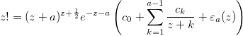
where a is an arbitrary positive integer that can be used to control the precision and the coefficients are given by

Factorial - Spouge's approximation - c0

Factorial - Spouge's approximation - ck

Please note that the coefficients are constants that only depend on a and not on the input argument to factorial.

The relative error when omitting the epsilon part is bound to

Factorial - Spouge's approximation - error

It is nice to have a function that defines the error, normally I need to empirically determine the error for a sensible range of input arguments and precision.

Expected error of Spouge’s Approximation

Lets implement the error formula and see how it behaves.

public static BigDecimal errorOfFactorialUsingSpouge(int a, MathContext mc) {
        return pow(BigDecimal.valueOf(a), BigDecimal.valueOf(-0.5), mc).multiply(pow(TWO.multiply(pi(mc), mc), BigDecimal.valueOf(-a-0.5), mc), mc);
    }

Instead of plotting the error bounds directly, I determine the achievable precision using -log10(error).

Precision of Spouge's approximation

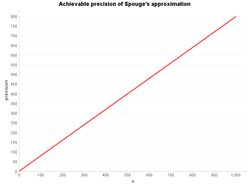
Using the relative error formula of Spouge’s approximation we see that the expected precision is pretty linear to the chosen value of a for the values [1..1000] (which are a sensible range for the precision the users of the function will use).

This will make it easy to calculate a sensible value for a from the desired precision.

Note: While testing this I found a bug in log(new BigDecimal("6.8085176335035800378E-325")). Fixed it before it could run away.

Caching Spouge’s coefficients (depending on precision)

The coefficients depend only on the value of a.

We can cache the coefficients for every value of a that we need:

private static Map<Integer, List<BigDecimal>> spougeFactorialConstantsCache = new HashMap<>();

    private static List<BigDecimal> getSpougeFactorialConstants(int a) {
        return spougeFactorialConstantsCache.computeIfAbsent(a, key -> {
            List<BigDecimal> constants = new ArrayList<>(a);
            MathContext mc = new MathContext(a * 15/10);

            BigDecimal c0 = sqrt(pi(mc).multiply(TWO, mc), mc);
            constants.add(c0);

            boolean negative = false;
            BigDecimal factor = c0;
            for (int k = 1; k < a; k++) {
                BigDecimal bigK = BigDecimal.valueOf(k);
                BigDecimal ck = pow(BigDecimal.valueOf(a-k), bigK.subtract(BigDecimal.valueOf(0.5), mc), mc);
                ck = ck.multiply(exp(BigDecimal.valueOf(a-k), mc), mc);
                ck = ck.divide(factorial(k - 1), mc);
                if (negative) {
                    ck = ck.negate();
                }
                constants.add(ck);

                negative = !negative;
            }

            return constants;
        });
    }

Calculating the coefficients becomes quite expensive with higher precision.

Time calculating Spouge's coefficients

This will need to be explained in the javadoc of the method.

Spouge’s approximation with pre-calculated constants

Now that we have the coefficients for a specific value of a we can implement the factorial method:

public static BigDecimal factorialUsingSpougeCached(BigDecimal x, MathContext mathContext) {
        MathContext mc = new MathContext(mathContext.getPrecision() * 2, mathContext.getRoundingMode());

        int a = mathContext.getPrecision() * 13 / 10;
        List<BigDecimal> constants = getSpougeFactorialConstants(a);

        BigDecimal bigA = BigDecimal.valueOf(a);

        boolean negative = false;
        BigDecimal factor = constants.get(0);
        for (int k = 1; k < a; k++) {
            BigDecimal bigK = BigDecimal.valueOf(k);
            factor = factor.add(constants.get(k).divide(x.add(bigK), mc), mc);
            negative = !negative;
        }

        BigDecimal result = pow(x.add(bigA, mc), x.add(BigDecimal.valueOf(0.5), mc), mc);
        result = result.multiply(exp(x.negate().subtract(bigA, mc), mc), mc);
        result = result.multiply(factor, mc);

        return result.round(mathContext);
    }

Let’s calculate first the factorial function with constant precision over a range of input values.

Time calculating Spouge's approximation with precalculated coefficients to precision of 200 digits

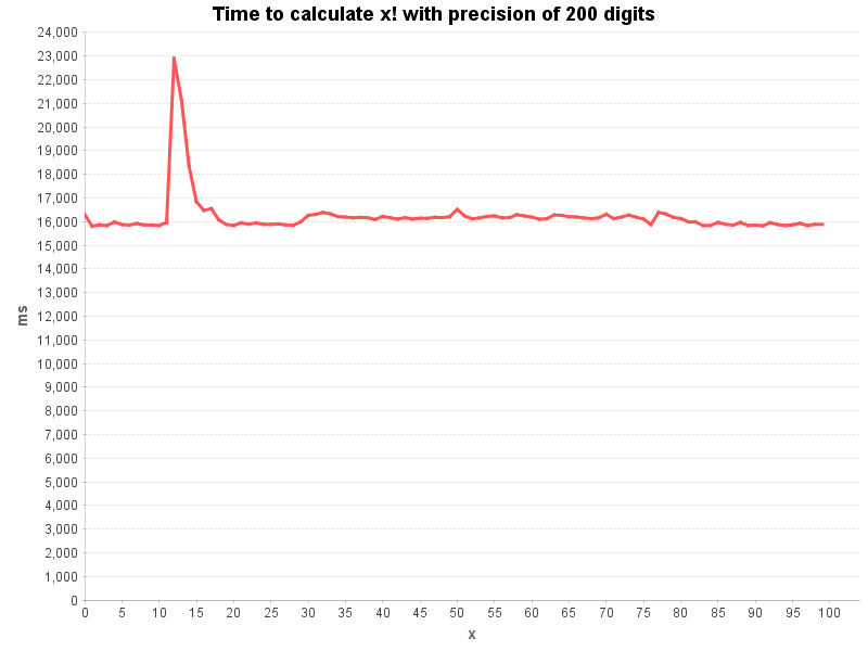
Looks like the argument x does not have much influence on the calculation time.

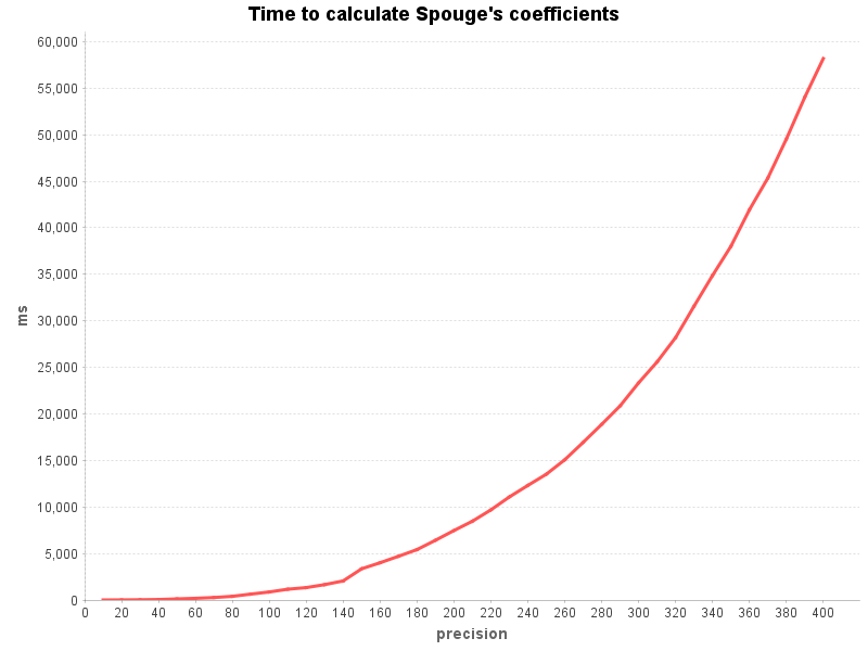
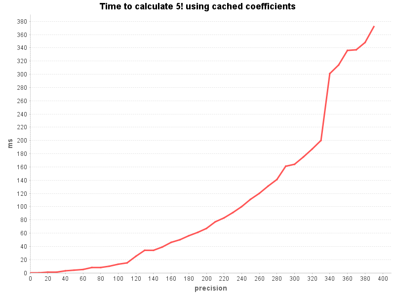
More interesting is the influence that the precision has on the calculation time. The following chart was measured by calculating 5! over a range of precisions:

Time calculating Spouge's approximation with precalculated coefficients to various precisions

Gamma function

The implementation of the Gamma function is trivial, now that we have a running factorial function.

public static BigDecimal gamma(BigDecimal x, MathContext mathContext) {
        return factorialUsingSpougeCached(x.subtract(ONE), mathContext);
    }

Polishing before adding it to BigDecimalMath

Before committing the new methods factorial() and gamma() to BigDecimalMath I need to do some polishing…

The access to the cache must be synchronized to avoid race conditions.

Most important is optimizing the calculation for the special cases of x being integer values which can be calculated much faster by calling BigDecimalMath.factorial(int).

Lots of unit tests of course! As usual Wolfram Alpha provides some nice reference values to prove that the calculations are correct (at least for the tested cases).

Writing javadoc takes also some time (and thoughts).

You can check out the final version in github: BigComplexMath.java

Posted in Development, Java, Math | Leave a comment

Release 2.0.0 of big-math library supports now complex numbers

The easter week-end was the perfect time to polish and release version 2.0.0 of the big-math library.

The class BigComplex represents complex numbers in the form (a + bi).
It follows the design of BigComplex with some convenience improvements like overloaded operator methods.

  • re
  • im
  • add(BigComplex)
  • add(BigComplex, MathContext)
  • add(BigDecimal)
  • add(BigDecimal, MathContext)
  • add(double)
  • subtract(BigComplex)
  • subtract(BigComplex, MathContext)
  • subtract(BigDecimal)
  • subtract(BigDecimal, MathContext)
  • subtract(double)
  • multiply(BigComplex)
  • multiply(BigComplex, MathContext)
  • multiply(BigDecimal)
  • multiply(BigDecimal, MathContext)
  • multiply(double)
  • divide(BigComplex)
  • divide(BigComplex, MathContext)
  • divide(BigDecimal)
  • divide(BigDecimal, MathContext)
  • divide(double)
  • reciprocal(MathContext)
  • conjugate()
  • negate()
  • abs(MathContext)
  • angle(MathContext)
  • absSquare(MathContext)
  • isReal()
  • re()
  • im()
  • round(MathContext)
  • hashCode()
  • equals(Object)
  • strictEquals(Object)
  • toString()
  • valueOf(BigDecimal)
  • valueOf(double)
  • valueOf(BigDecimal, BigDecimal)
  • valueOf(double, double)
  • valueOfPolar(BigDecimal, BigDecimal, MathContext)
  • valueOfPolar(double, double, MathContext)

A big difference to BigDecimal is that BigComplex.equals() implements the mathematical equality and not the strict technical equality.
This was a difficult decision because it means that BigComplex behaves slightly different than BigDecimal but considering that the strange equality of BigDecimal is a major source of bugs we decided it was worth the slight inconsistency.

If you need the strict equality use BigComplex.strictEquals().

The class BigComplexMath is the equivalent of BigDecimalMath and contains mathematical functions in the complex domain.

  • sin(BigComplex, MathContext)
  • cos(BigComplex, MathContext)
  • tan(BigComplex, MathContext)
  • asin(BigComplex, MathContext)
  • acos(BigComplex, MathContext)
  • atan(BigComplex, MathContext)
  • acot(BigComplex, MathContext)
  • exp(BigComplex, MathContext)
  • log(BigComplex, MathContext)
  • pow(BigComplex, long, MathContext)
  • pow(BigComplex, BigDecimal, MathContext)
  • pow(BigComplex, BigComplex, MathContext)
  • sqrt(BigComplex, MathContext)
  • root(BigComplex, BigDecimal, MathContext)
  • root(BigComplex, BigComplex, MathContext)
Posted in Development, Java, Math | Leave a comment

Aurora Borealis (Northern Lights) in Tromsø

To celebrate my fiftieth birthday the whole family had a great vacation in Tromsø to see the northern lights.

The following videos where all taken using a wireless remote control with programmable interval.


The single shots where joined using ffmpeg.

#!/bin/sh
# $1 = framerate (for aurora timelapse use 1 to 4)
# $2 = start number of first image
# $3 = output file (with .mp4 extension)

ffmpeg -y -r "$1" -start_number "$2" -i IMG_%04d.JPG -s hd1080 -vf "framerate=fps=30:interp_start=0:interp_end=255:scene=100" -vcodec mpeg4 -q:v 1 "$3

In a few cases the images where a bit underexposed and needed to be brightened.
This was done with a simple shell script using the imagemagick convert.

#!/bin/sh

mkdir modulate150

for i in *.JPG
do
        convert $i -modulate 150% modulate150/$i
done
Posted in Photography, Timelapse | Leave a comment

Adaptive precision in Newton’s Method

This describes a way to improve the performance of a BigDecimal based implementation of Newton’s Method
by adapting the precision for every iteration to the maximum precision that is actually possible at this step.

As showcase I have picked the implementation of Newton’s Method to calculate the natural logarithm of a BigDecimal value with a determined precision.

The source code is available on github: big-math.

Here the mathematical formulation of the algorithm:

\(\require{AMSmath}\)
\(\displaystyle y_0 = \operatorname{Math.log}(x),\)
\(\displaystyle y_{i+1} = y_i + 2 \frac{x – e^{y_i} }{ x + e^{y_i}},\)
\(\displaystyle \ln{x} = \lim_{i \to \infty} y_i\)

Here a straightforward implementation:

private static final BigDecimal TWO = valueOf(2);

public static BigDecimal logUsingNewtonFixPrecision(BigDecimal x, MathContext mathContext) {
	if (x.signum() <= 0) {
		throw new ArithmeticException("Illegal log(x) for x <= 0: x = " + x);
	}

	MathContext mc = new MathContext(mathContext.getPrecision() + 4, mathContext.getRoundingMode());
	BigDecimal acceptableError = BigDecimal.ONE.movePointLeft(mathContext.getPrecision() + 1);
	
	BigDecimal result = BigDecimal.valueOf(Math.log(x.doubleValue()));
	BigDecimal step;
	
	do {
		BigDecimal expY = BigDecimalMath.exp(result, mc); // available on https://github.com/eobermuhlner/big-math
		step = TWO.multiply(x.subtract(expY, mc), mc).divide(x.add(expY, mc), mc);
		result = result.add(step);
	} while (step.abs().compareTo(acceptableError) > 0);

	return result.round(mathContext);
}

The MathContext mc is created with a precision of 4 digits more than the output is expected to have.
All calculations are done with this MathContext and therefore with the full precision.

The result is correct but we can improve the performance significantly be adapting the precision for every iteration.

The initial approximation uses Math.log(x.doubleValue()) which has a precision of about 17 significant digits.

We can expect that the precision triples with every iteration so it does not make sense to calculate with a higher precision than necessary.

Here the same implementation with a temporary MathContext that is recreated with a different precision every iteration.

public static BigDecimal logUsingNewtonAdaptivePrecision(BigDecimal x, MathContext mathContext) {
	if (x.signum() <= 0) {
		throw new ArithmeticException("Illegal log(x) for x <= 0: x = " + x);
	}

	int maxPrecision = mathContext.getPrecision() + 4;
	BigDecimal acceptableError = BigDecimal.ONE.movePointLeft(mathContext.getPrecision() + 1);
	
	BigDecimal result = BigDecimal.valueOf(Math.log(x.doubleValue()));
	int adaptivePrecision = 17;
	BigDecimal step = null;
	
	do {
		adaptivePrecision = adaptivePrecision * 3;
		if (adaptivePrecision > maxPrecision) {
			adaptivePrecision = maxPrecision;
		}
		MathContext mc = new MathContext(adaptivePrecision, mathContext.getRoundingMode());
		
		BigDecimal expY = BigDecimalMath.exp(result, mc); // available on https://github.com/eobermuhlner/big-math
		step = TWO.multiply(x.subtract(expY, mc), mc).divide(x.add(expY, mc), mc);
		result = result.add(step);
	} while (adaptivePrecision < maxPrecision || step.abs().compareTo(acceptableError) > 0);

	return result.round(mathContext);
}

The performance comparison between the two implementations is impressive.
The following chart shows the time in nanoseconds it takes to calculate the log() of values of x in the range from 0 to 1 with a precision of 300 digits.

Here some more charts to show the performance improvements of the adaptive precision technique applied to different approximative implementations:


This method can only be applied to approximative methods that improve the result with every iteration and discard the previous result, such as Newton’s Method.

It does obviously not work on methods that accumulate the results of each iteration to calculate the final result, such as Taylor series which add the terms.

Posted in Development, Java, Math | Leave a comment

BigDecimalMath

\(\require{AMSmath}\)
Java 8 is out and there are still no Math functions for BigDecimal.

After playing around with some implementations to calculate Pi I decided to write some implementation of BigDecimalMath to fill this gap.

The result of this is available on github: big-math.

The goal was to provide the following functions:

  • exp(x)
  • log(x)
  • pow(x, y)
  • sqrt(x)
  • root(n, x)
  • sin(x), cos(x), tan(x), cot(x)
  • asin(x), acos(x), atan(x), acot(x)
  • sinh(x), cosh(x), tanh(x)
  • asinh(x), acosh(x), atanh(x)

The calculations must be accurate to the desired precision (specified in the MathContext)
and the performance should be acceptable and stable for a large range of input values.

Implementation Details

Implementation exp(x)

To implement exp() the classical Taylor series was used:
\(\displaystyle e^x = \sum^{\infty}_{n=0} \frac{x^n}{n!} = 1 + x + \frac{x^2}{2!} + \frac{x^3}{3!} + \cdots\)

Implementation log()

Note that in Java the function name log() means the natural logarithm, which in mathematical notation is written \(\ln{x}\).

The implementation of log() is based on Newton’s method.
We can use the double version Math.log() to give us a good initial value.

\(\displaystyle y_0 = \operatorname{Math.log}(x),\)
\(\displaystyle y_{i+1} = y_i + 2 \frac{x – e^{y_i} }{ x + e^{y_i}},\)
\(\displaystyle \ln{x} = \lim_{i \to \infty} y_i\)

Several optimizations in the implementation transform the argument of log(x) so that it will be nearer to the optimum of 1.0 to converge faster.
\(
\begin{align}
\displaystyle \ln{x} & = \ln{\left(a \cdot 10^b\right)} = \ln{a} + \ln{10} \cdot b & \qquad \text{for } x \leq 0.1 \text{ or } x \geq 10 \\
\displaystyle \ln{x} & = \ln{\left( 2 x \right)} – \ln{2} & \qquad \text{for } x \lt 0.115 \\
\displaystyle \ln{x} & = \ln{\left( 3 x \right)} – \ln{3} & \qquad \text{for } x \lt 0.14 \\
\displaystyle \ln{x} & = \ln{\left( 4 x \right)} – 2 \ln{2} & \qquad \text{for } x \lt 0.2 \\
\displaystyle \ln{x} & = \ln{\left( 6 x \right)} – \ln{2} – \ln{3} & \qquad \text{for } x \lt 0.3 \\
\displaystyle \ln{x} & = \ln{\left( 8 x \right)} – 3 \ln{2} & \qquad \text{for } x \lt 0.42 \\
\displaystyle \ln{x} & = \ln{\left( 9 x \right)} – 3 \ln{3} & \qquad \text{for } x \lt 0.7 \\
\displaystyle \ln{x} & = \ln{\left( \frac{1}{2} x \right)} + \ln{2} & \qquad \text{for } x \lt 2.5 \\
\displaystyle \ln{x} & = \ln{\left( \frac{1}{3} x \right)} + \ln{3} & \qquad \text{for } x \lt 3.5 \\
\displaystyle \ln{x} & = \ln{\left( \frac{1}{4} x \right)} + 2 \ln{2} & \qquad \text{for } x \lt 5.0 \\
\displaystyle \ln{x} & = \ln{\left( \frac{1}{6} x \right)} + \ln{2} + \ln{3} & \qquad \text{for } x \lt 7.0 \\
\displaystyle \ln{x} & = \ln{\left( \frac{1}{8} x \right)} + 3 \ln{2} & \qquad \text{for } x \lt 8.5 \\
\displaystyle \ln{x} & = \ln{\left( \frac{1}{9} x \right)} + 3 \ln{3} & \qquad \text{for } x \lt 10.0
\end{align}
\)

The additional logarithmic functions to different common bases are simple:
\(\displaystyle \operatorname{log}_2{x} = \frac{\ln{x}}{\ln{2}}\)

\(\displaystyle \operatorname{log}_{10}{x} = \frac{\ln{x}}{\ln{10}}\)

Since the precalculated values for \(\ln{2}, \ln{3}, \ln{10}\) with a precision of up to 1100 digits already exist for the optimizations mentioned above, the log2() and log10() functions could reuse them and are therefore reasonably fast.

Implementation pow(x)

The implementation of pow() with non-integer arguments is based on exp() and log():

\(\displaystyle x^y = e^{y \ln x}\)

If y is an integer argument then pow() is implemented with multiplications:

\(\displaystyle x^y = \prod_{i \to y} x\)

Actually the implementation is further optimized to reduce the number of multiplications by squaring the argument whenever possible.

Implementation sqrt(x), root(n, x)

The implementation of sqrt() and root() uses Newton’s method to approximate the result until the necessary precision is reached.
In the case of sqrt() we can use the double version Math.sqrt() to give us a good initial value.

\(\displaystyle y_0 = \operatorname{Math.sqrt}(x),\)
\(\displaystyle y_{i+1} = \frac{1}{2} \left(y_i + \frac{x}{y_i}\right),\)
\(\displaystyle \sqrt{x} = \lim_{i \to \infty} y_i\)

Unfortunately the root() function does not exist for double so we are forced to use a simpler initial value.

\(\displaystyle y_0 = \frac{1}{n},\)
\(\displaystyle y_{i+1} = \frac{1}{n} \left[{(n-1)y_i +\frac{x}{y_i^{n-1}}}\right],\)
\(\displaystyle \sqrt[n]{x} = \lim_{i \to \infty} y_i\)

Implementation sin(x), cos(x), tan(x), cot(x)

The basic trigonometric functions where implemented using Taylor series or if this proved more efficient by their relationship with an already implemented functions:

\(\displaystyle \sin x = \sum^{\infty}_{n=0} \frac{(-1)^n}{(2n+1)!} x^{2n+1} = x – \frac{x^3}{3!} + \frac{x^5}{5!} – \cdots\)

\(\displaystyle \cos x = \sum^{\infty}_{n=0} \frac{(-1)^n}{(2n)!} x^{2n} = 1 – \frac{x^2}{2!} + \frac{x^4}{4!} – \cdots\)

\(\displaystyle \tan x = \frac{\sin x}{\cos x}\)

\(\displaystyle \cot x = \frac{\cos x}{\sin x}\)

Implementation asin(x), acos(x), atan(x), acot(x)

The inverse trigonometric functions use a Taylor series for arcsin().

\(\displaystyle \arcsin x = \sum^{\infty}_{n=0} \frac{(2n)!}{4^n (n!)^2 (2n+1)} x^{2n+1}\)

This series takes very long to converge, especially when the argument x gets close to 1.
As optimization the argument x is transformed to a more efficient range using the following relationship.

\(\displaystyle \arcsin x = \arccos \sqrt{1-x^2} \qquad \text{for } x \gt \sqrt{\frac{1}{2}} \text{ (} \approx 0.707107 \text{)}\)

The remaining functions are implemented by their relationship with arcsin().

\(\displaystyle \arccos x = \frac{\pi}{2} – \arcsin x\)

\(\displaystyle \arctan x = \arcsin \frac{x}{\sqrt{1+x^2}}\)

\(\displaystyle \operatorname{arccot} x = \frac{\pi}{2} – \arctan x\)

Implementation sinh(x), cosh(x), tanh(x)

Taylor series are efficient for most of the implementations of hyperbolic functions.

\(\displaystyle \sinh x= \sum_{n=0}^\infty \frac{x^{2n+1}}{(2n+1)!} = x + \frac{x^3}{3!} + \frac{x^5}{5!} + \frac{x^7}{7!} +\cdots\)

\(\displaystyle \cosh x = \sum_{n=0}^\infty \frac{x^{2n}}{(2n)!} = 1 + \frac{x^2}{2!} + \frac{x^4}{4!} + \frac{x^6}{6!} + \cdots\)

The Taylor series for tanh() converges very slowly, so we use the relationship with sinh() and tanh() instead.
\(\displaystyle \tanh x = \frac{\sinh x}{\cosh x}\)

Implementation asinh(x), acosh(x), atanh(x)

The inverse hyperbolic functions can be expressed using natural logarithm.

\(\displaystyle \operatorname{arsinh} x = \ln(x + \sqrt{x^2 + 1} )\)

\(\displaystyle \operatorname{arcosh} x = \ln(x + \sqrt{x^2-1} )\)

\(\displaystyle \operatorname{artanh} x = \frac12\ln\left(\frac{1+x}{1-x}\right)\)

Performance calculating different precisions

Obviously it will take longer to calculate a function result with a higher precision than a lower precision.

The following charts show the time needed to calculate the functions with different precisions.

The arguments of the functions where:

  • log(3.1)
  • exp(3.1)
  • pow(123.456, 3.1)
  • sqrt(3.1)
  • root(2, 3.1)
  • root(3, 3.1)
  • sin(3.1)
  • cos(3.1)


While the time to calculate the results grows worse than linear for higher precisions the speed is still reasonable for precisions of up to 1000 digits.

Performance calculating different values

The following charts show the time needed to calculate the functions over a range of values with a precision of 300 digits.

  • log(x)
  • exp(x)
  • pow(123.456, x)
  • sqrt(x)
  • root(2, x)
  • root(3, x)
  • sin(x)
  • cos(x)

The functions have been separated in a fast group (exp, sqrt, root, sin, cos) and a slow group (exp, log, pow).
For comparison reasons the exp() function is contained in both groups.

Range 0 to 2


The performance of the functions is in a reasonable range and is stable, especially when getting close to 0 in which some functions might converge slowly.
The functions exp(), sin(), cos() need to be watched at the higher values of x to prove that the do not continue to grow.

Shows nicely that log() is more efficient when x is close to 1.0.
By using divisions and multiplication with the prime numbers 2 and 3 the log() function was optimized to use this fact for values of x than can be brought closer to 1.0.
This gives the strange arches in the performance of log().
The pow() function performs fairly constant, except for the powers of integer values which are optimized specifically.

Range 0 to 10


Shows that sin(), cos() have been optimized with the period of 2*Pi (roughly 6.28) so that they do not continue to grow with higher values.
This optimization has some cost which needs to be watched at higher values.


exp() has become stable and does no longer grow.
log() is stable and shows the typical arches with optimas at 1.0, 2.0 (divided by 2), 3.0 (divided by 3), 4.0 (divided by 2*2), 6.0 (divided by 2*3), 8.0 (divided by 2*2*2) and 9.0 (divided by 3*3).
pow() continues stable.

Range -10 to 10


Positive and negative values are symmetric for all functions that are defined for the negative range.

Range 0 to 100


All functions are stable over this range.


All functions are stable over this range.
The pow() function makes the chart somewhat hard to read because of the optimized version for integer powers.
The log() function shows here the effect of another optimization using the expoential form. The range from 10 to 100 is brought down to the range 1 to 10 and the same divisions are applied. This has the effect of showing the same arches again in the range from 10 to 100.

Posted in Development, Java, Math | Tagged , , , , , , , | 8 Comments

Bernoulli Numbers

As part of the ongoing development of the BigRational and BigDecimalMath classes I needed to implement a method to calculate the Bernoulli numbers.

Since I had a hard time to find a reference list of the Bernoulli numbers I will put the table of the first few calculated numbers here.

For a larger list of Bernoulli numbers have a look at the bernoulli.csv file.

B0 =
1

B1 =
 -1 
 2 

B2 =
 1 
 6 

B3 =
0

B4 =
 -1 
 30 

B5 =
0

B6 =
 1 
 42 

B7 =
0

B8 =
 -1 
 30 

B9 =
0

B10 =
 5 
 66 

B11 =
0

B12 =
 -691 
 2730 

B13 =
0

B14 =
 7 
 6 

B15 =
0

B16 =
 -3617 
 510 

B17 =
0

B18 =
 43867 
 798 

B19 =
0

B20 =
 -174611 
 330 

B21 =
0

B22 =
 854513 
 138 

B23 =
0

B24 =
 -236364091 
 2730 

B25 =
0

B26 =
 8553103 
 6 

B27 =
0

B28 =
 -23749461029 
 870 

B29 =
0

B30 =
 8615841276005 
 14322 

B31 =
0

B32 =
 -7709321041217 
 510 

B33 =
0

B34 =
 2577687858367 
 6 

B35 =
0

B36 =
 -26315271553053477373 
 1919190 

B37 =
0

B38 =
 2929993913841559 
 6 

B39 =
0

B40 =
 -261082718496449122051 
 13530 

B41 =
0

B42 =
 1520097643918070802691 
 1806 

B43 =
0

B44 =
 -27833269579301024235023 
 690 

B45 =
0

B46 =
 596451111593912163277961 
 282 

B47 =
0

B48 =
 -5609403368997817686249127547 
 46410 

B49 =
0

B50 =
 495057205241079648212477525 
 66 

B51 =
0

B52 =
 -801165718135489957347924991853 
 1590 

B53 =
0

B54 =
 29149963634884862421418123812691 
 798 

B55 =
0

B56 =
 -2479392929313226753685415739663229 
 870 

B57 =
0

B58 =
 84483613348880041862046775994036021 
 354 

B59 =
0

B60 =
 -1215233140483755572040304994079820246041491 
 56786730 

B61 =
0

B62 =
 12300585434086858541953039857403386151 
 6 

B63 =
0

B64 =
 -106783830147866529886385444979142647942017 
 510 

B65 =
0

B66 =
 1472600022126335654051619428551932342241899101 
 64722 

B67 =
0

B68 =
 -78773130858718728141909149208474606244347001 
 30 

B69 =
0

B70 =
 1505381347333367003803076567377857208511438160235 
 4686 

B71 =
0

B72 =
 -5827954961669944110438277244641067365282488301844260429 
 140100870 

B73 =
0

B74 =
 34152417289221168014330073731472635186688307783087 
 6 

B75 =
0

B76 =
 -24655088825935372707687196040585199904365267828865801 
 30 

B77 =
0

B78 =
 414846365575400828295179035549542073492199375372400483487 
 3318 

B79 =
0

Posted in Development, Math | Leave a comment

Using GLSL to generate gas giant planets

To be completely honest, the code that is described in this blog is already more than a year old. I just wanted to catch up with the current state of my project. I will therefore try to write several blogs in the next couple of days describing what has been going on…

After my first experiments with earth-like planets I wanted to experiment with creating Jupiter-like gas giants in GLSL.

The approach is still noise based but instead of creating a height map we now want to create something that looks like turbulent clouds.

The following scr