Using GLSL Shaders to generate Planets

My goal was to write a GLSL shader that would create an earth-like planet.

There are lots of good introductions into GLSL shader programming.

• Creating a Shader with LibGDX from Xoppa
• Lighthouse3d – GLSL Tutorial

The following example is based on LibGDX, but it should be easily adapted to another framework.

First we need a little program so that we can experiment with the shader programs and see the results.

public class ShaderTest extends ApplicationAdapter {
	private ModelBatch modelBatch;

	private PerspectiveCamera camera;
	private CameraInputController cameraInputController;
	private Environment environment;

	private final ModelBuilder modelBuilder = new ModelBuilder();
	private final Array instances = new Array();

	private static final int SPHERE_DIVISIONS_U = 20;
	private static final int SPHERE_DIVISIONS_V = 20;

	@Override
	public void create () {
		createTest(new UberShaderProvider("planet")), new Material(), Usage.Position | Usage.Normal | Usage.TextureCoordinates);
	}

	private void createTest(ShaderProvider shaderProvider, Material material, long usageAttributes) {
		modelBatch = new ModelBatch(shaderProvider);

		camera = new PerspectiveCamera(67, Gdx.graphics.getWidth(), Gdx.graphics.getHeight());
		camera.position.set(10f, 10f, 10f);
		camera.lookAt(0, 0, 0);
		camera.near = 1f;
		camera.far = 300f;
		camera.update();

		cameraInputController = new CameraInputController(camera);
		Gdx.input.setInputProcessor(cameraInputController);

		environment = new Environment();
		environment.set(new ColorAttribute(ColorAttribute.AmbientLight, Color.DARK_GRAY));
		environment.add(new DirectionalLight().set(Color.WHITE, 20, -10, -10));

		float sphereRadius = 15f;
		Model model = modelBuilder.createSphere(sphereRadius, sphereRadius, sphereRadius, SPHERE_DIVISIONS_U, SPHERE_DIVISIONS_V, material, usageAttributes);

		ModelInstance instance = new ModelInstance(model);
		instances.add(instance);
	}

	@Override
	public void render () {
		Gdx.gl.glViewport(0, 0, Gdx.graphics.getWidth(), Gdx.graphics.getHeight());
		Gdx.gl.glClearColor(0.0f, 0.0f, 0.8f, 1.0f);
		Gdx.gl.glClear(GL20.GL_COLOR_BUFFER_BIT | GL20.GL_DEPTH_BUFFER_BIT);

		cameraInputController.update();

		modelBatch.begin(camera);
		modelBatch.render(instances, environment);
		modelBatch.end();
	}
}

public class UberShaderProvider extends BaseShaderProvider {

	private String shaderName;

	public UberShaderProvider (String shaderName) {
		this.shaderName = shaderName;
	}

	@Override
	protected Shader createShader(Renderable renderable) {
		String vert = Gdx.files.internal("data/shaders/" + shaderName + ".vertex.glsl").readString();
		String frag = Gdx.files.internal("data/shaders/" + shaderName + ".fragment.glsl").readString();
		return new DefaultShader(renderable, new DefaultShader.Config(vert, frag));
	}

}

Now we can simply replace the string argument to the UberShaderProvider to test a particular pair of vertex and fragment shader programs in
the assets folder data/shaders/.

Simple Vertex Shader

First we will need a simple vertex shader that transforms the local vertex position into a global position and
passes the texture coordinates on to the fragment shader.

attribute vec3 a_position;
attribute vec2 a_texCoord0;

uniform mat4 u_worldTrans;
uniform mat4 u_projViewTrans;

varying vec2 v_texCoords0;

void main() {
	v_texCoords0 = a_texCoord0;

	gl_Position = u_projViewTrans * u_worldTrans * vec4(a_position, 1.0);
}

Simple Fragment Shader

Now we can write the fragment shader.

Let’s start by calculating a color directly from the texture coordinates.

Since you typically have no debuggers for shader programs the easiest way to figure out what is going on is to visualize the intermediate steps as colors.
With some experience you will be able to see the values just by looking at the rendered graphics.

#ifdef GL_ES 
#define LOWP lowp
#define MED mediump
#define HIGH highp
precision mediump float;
#else
#define MED
#define LOWP
#define HIGH
#endif

varying MED vec2 v_texCoords0;

void main() {
	vec3 color = vec3(v_texCoords0.x, v_texCoords0.y, 0.0);

	gl_FragColor.rgb = color;
}

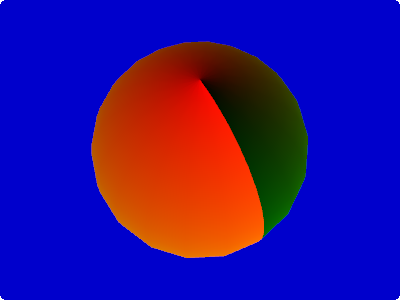
You can see that the x coordinate of the texture is mapped to the red color of each pixel.
The y coordinate of the texture is mapped to the green color of each pixel.

Convert noise into colors

The next step is to use a noise function that we will then use to create the pseudo-random oceans and continents.

You can find an excellent noise function in the webgl-noise project.

Copy and paste the source code from the file noise2D.glsl into your shader.

#ifdef GL_ES 
#define LOWP lowp
#define MED mediump
#define HIGH highp
precision mediump float;
#else
#define MED
#define LOWP
#define HIGH
#endif

varying MED vec2 v_texCoords0;

// INSERT HERE THE NOISE FUNCTIONS ...

float pnoise2(vec2 P, float period) {
	return pnoise(P*period, vec2(period, period));
}

float earthNoise(vec2 P) {
	vec2 r1 = vec2(0.70, 0.82); // random numbers

	float noise = 0.0; 
	noise += pnoise2(P+r1, 9.0);
	
	return noise;
}

void main() {
	float noise = earthNoise(v_texCoords0);

	gl_FragColor.rgb = noise;
}

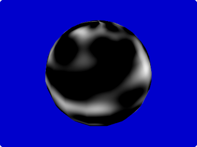
Obviously the noise value 1.0 corresponds to white (= vec3(1.0, 1.0, 1.0)), while noise value 0.0 corresponds to black (= vec3(0.0, 0.0, 0.0)).
By now you might be wondering why the black areas are so large – is the noise function faulty?
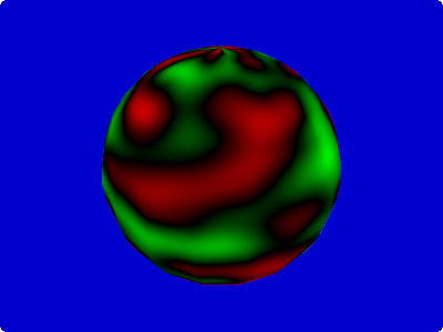
Actually the noise function returns values in the range -1.0 to 1.0. But the conversion to RGB colors clamps all negative values to 0.0, hence the large black areas.

As an exercise to prove this (and as a tool to debug negative values in the future) let’s write a function that converts positive values (0.0 to 1.0) into green colors and negative values (-1.0 to 0.0) into red colors.

// lots of code omitted ...

vec3 toColor(float value) {
	float r = clamp(-value, 0.0, 1.0);
	float g = clamp(value, 0.0, 1.0);
	float b = 0.0;
	return vec3(r, g, b);
}

void main() {
	float noise = earthNoise(v_texCoords0);

	gl_FragColor.rgb = toColor(noise);
}

Hint: Try to avoid constructs using if because the GPU doesn’t like branching.
Instead of using if branching you should try to implement your functionality with the provided mathematical functions (clamp, mix, step, smoothstep, … ).
For a useful reference see: OpenGL ES Shading Language Built-In Functions

Convert height into colors

We want to treat the result of the noise function as the height of the planet and map this height into the typical colors.
The easiest way to implement a function of an input value into a color is to use a one-dimensional texture.

The x-axis of the texture corresponds to the height of the planet.

Until about 0.45 we paint all the heights the same deep blue of the ocean, then a few pixels of turquoise for the coastal waters, various green and yellows for the flora and deserts closer to the coast, then a large dark green block for the deep forest, finishing the whole with some grey mountains and a single white pixel for the snow at the top.

In the java code that defines the material we need now to specify this texture.

		createTest(new UberShaderProvider("planet_step3"), new Material(new TextureAttribute(TextureAttribute.Diffuse, new Texture("data/textures/planet_height_color.png"))), Usage.Position | Usage.Normal | Usage.TextureCoordinates);

// lots of code omitted ...

void main() {
	float noise = earthNoise(v_texCoords0);

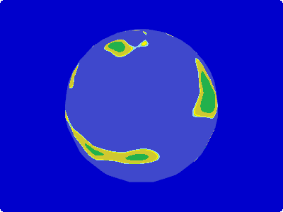
	vec3 color = texture2D(u_diffuseTexture, vec2(clamp(noise, 0.0, 1.0), 0.0));

	gl_FragColor.rgb = color;
}

We do a lookup with texture2D() using the noise value as x-coordinate of the texture.
This looks already pretty reasonable.

Tweak the noise frequencies

Now it is time to make our continents a bit more convincing.
We want a couple of big continents with coastal areas that vary from smooth like the coasts of south-western Africa to fragmented like the fjords of Norway.

After some experiments I liked the following result:

float earthNoise(vec2 P) {
	vec2 r1 = vec2(0.70, 0.82);
	vec2 r2 = vec2(0.81, 0.12);
	vec2 r3 = vec2(0.24, 0.96);
	vec2 r4 = vec2(0.39, 0.48);
	vec2 r5 = vec2(0.02, 0.25);
	vec2 r6 = vec2(0.77, 0.91);
	vec2 r7 = vec2(0.48, 0.05);
	vec2 r8 = vec2(0.82, 0.48);

	float noise = 0.0; 
	noise += clamp(pnoise2(P+r1, 3.0), 0.0, 0.45); // low-frequency noise clamped just slightly above ocean level - this produces the continental plates
	noise += pnoise2(P+r2, 9) * 0.7; // medium frequency noise to produce the high mountain ranges (can be under and above water)
	noise += pnoise2(P+r3, 14) * 0.2 + 0.1; // medium frequency noise for some hilly regious
	noise += smoothstep(0.0, 0.1, pnoise2(P+r4, 8.0)) * pnoise2(P+r5, 50.0) * 0.3; // high frequency noise - but not in all areas
	noise += smoothstep(0.0, 0.1, pnoise2(P+r6, 11.0)) * pnoise2(P+r7, 500.0) * 0.01;  // very high frequency noise - but not in all areas
	noise += smoothstep(0.8, 1.0, noise) * pnoise2(P+r8, 350.0) * -0.3;  // very high frequency noise - only in the highest mountains
	
	return noise;
}

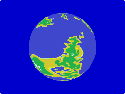
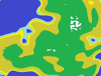
The vectors r1 to r8 are random numbers so that not all our generated planets will look the same.
Later we can make then into uniforms and control them from the Java application.

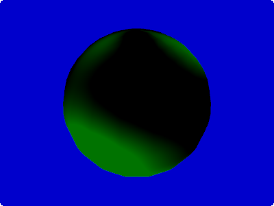
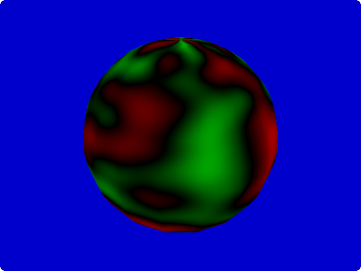
If you want to understand how the different noise parts contribute to the total noise you can use the toColor() function to debug it visually.
Comment out all the other noise components and feed the final result into toColor().

	noise += clamp(pnoise2(P+r1, 3.0), 0.0, 0.45); // low-frequency noise clamped just slightly above ocean level - this produces the continental plates

	noise += pnoise2(P+r2, 9) * 0.7; // medium frequency noise to produce the high mountain ranges (can be under and above water)

	noise += pnoise2(P+r3, 14) * 0.2 + 0.1; // medium frequency noise for some hilly regious

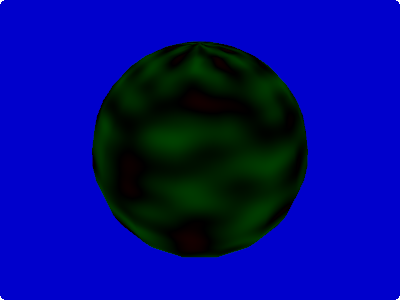
	noise += smoothstep(0.0, 0.1, pnoise2(P+r4, 8.0)) * pnoise2(P+r5, 50.0) * 0.3; // high frequency noise - but not in all areas

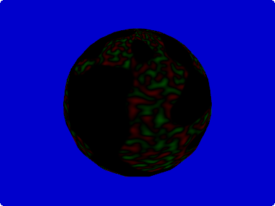
The very high frequency with an amplitute of 0.01 is not visible with the color range of our toColor() function
and the last smoothstep() uses the calculated noise so that only the high mountain ranges receive the high frequency noise.
If you want to make these visible you need play around with the functions.

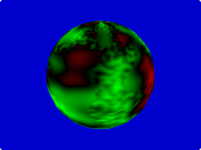
As last step lets have a look at the total output of the noise function using toColor().

Convert latitude and height into colors

Our planet already looks reasonable but if you look at a picture of earth you will immediately notice that the latitude also influences the color.
High in the north and south we have the polar caps and closer to the equator we see large desert areas.

To implement this we can use a 2 dimensional texture.

As before it encodes in the x-axis the height of the plant, on the y-axis corresponds to the distance to the equator.

We see the desert and steppe close to the equator. In the medium latitudes forest becomes predominant before it is replaced by tundra and finally the ice cap at the pole.

Let’s do the two-dimensional lookup in this texture.

void main() {
	float noise = earthNoise(v_texCoords0);

	float distEquator = abs(v_texCoords0.t - 0.5) * 2.0;
	vec3 color = texture2D(u_diffuseTexture, vec2(clamp(noise, 0.0, 1.0), distEquator));

	gl_FragColor.rgb = color;
}

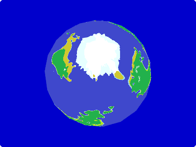
By changing the calculation of the distance to equator we can change the overall climate of the planet.
Let’s have a look how it looks during an ice age.

void main() {
	float distEquator = abs(v_texCoords0.t - 0.5) * 6.0;
}

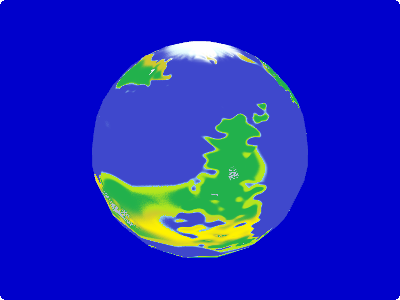
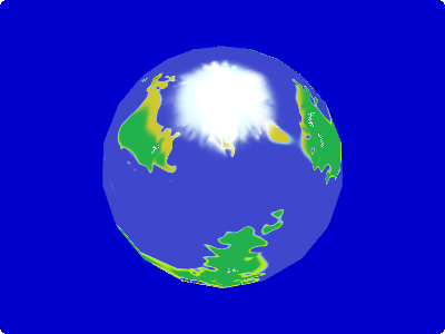
Actually we can make the whole planet look much nicer by running a gaussian blur over the texture, so that the colors of the different bio zones mix with each other.
Please note that the coast is not blurred into the water.

Here some more screenshots using the blurred texture.